Understanding Naive Bayes: Conditional Probability, Shopping Decisions, and Spam Classification
Learn how Naive Bayes combines priors and likelihoods, with complete shopping and spam examples, an interactive classifier, Laplace smoothing, and practical model checks.
Will a customer buy when a shop offers a discount and free delivery? Does a short comment belong in the spam folder? Naive Bayes approaches these classification questions by combining class frequencies with the evidence supplied by individual features.
The useful part is seeing exactly how those quantities combine. We will calculate a shopping prediction from frequency tables, then classify a short comment using word counts. Along the way, we will distinguish raw scores from normalized probabilities and see why smoothing matters.
Both examples are small teaching datasets. Their predictions illustrate the model's calculation, with no measured claim about accuracy on future customers or messages.
In this article: Bayes' theorem · The independence assumption · Shopping example · Interactive classifier · Smoothing · Spam example · Model variants · Evaluation · References
What is Naive Bayes?
Naive Bayes is a family of supervised probabilistic classifiers. Training estimates a class prior and a distribution for each feature within each class. Prediction combines those estimates to compare the possible class labels. 2
In the shopping example, the inputs are day type, discount availability, and free delivery. The target is a class label: Buy or No Buy. In the text example, word counts are the inputs, and the classes are Spam and Ham, where ham means a non-spam message.
Different members of the family use different feature distributions. Categorical Naive Bayes suits named categories such as day type. Multinomial Naive Bayes is commonly used with word counts. We will return to the other variants after the calculations.
Bayes' theorem: the starting point
Bayes' theorem connects the probability of a class before observing evidence with its probability after observing that evidence. For a class C and evidence x, with P(x) > 0:
P(C | x) = P(x | C)P(C)
           ────────────
               P(x)
| Quantity | Name | Meaning |
|---|---|---|
P(C) | Prior | Class probability before using this example's features |
| `P(x | C)` | Likelihood |
P(x) | Evidence | Overall probability of observing the evidence |
| `P(C | x)` | Posterior |
For example, P(Weekday | Buy) asks how often buying cases occur on weekdays. P(Buy | Weekday) asks how often weekday cases result in buying. The conditioning changes which group supplies the denominator. 1
A single-feature calculation
Suppose 30 shopping observations include 24 purchases and 6 non-purchases. Of the 11 weekday observations, 9 resulted in Buy and 2 in No Buy:
P(Buy)             = 24 / 30
P(No Buy)          =  6 / 30
P(Weekday)         = 11 / 30
P(Weekday | Buy)   =  9 / 24
P(Weekday | No Buy)=  2 / 6
Apply Bayes' theorem without rounding the inputs:
P(Buy | Weekday) = (9 / 24)(24 / 30) / (11 / 30)
                = 9 / 11
                ≈ 0.818181818

P(No Buy | Weekday) = (2 / 6)(6 / 30) / (11 / 30)
                   = 2 / 11
                   ≈ 0.181818182
The results sum to one. For this single feature, they are exactly the purchase frequencies within the observed weekday group: 81.82% Buy and 18.18% No Buy.
What makes the model naive?
With several features, the likelihood is a joint probability:
P(x₁, x₂, …, xₙ | C)
Naive Bayes assumes that the features are conditionally independent given the class, allowing the factorization:
P(x₁, x₂, …, xₙ | C) = ∏ⱼ P(xⱼ | C)
The condition “given the class” matters. The model estimates each feature's distribution separately inside Buy and inside No Buy. Features can still be related in the overall population, and actual data can violate the conditional independence assumption. 2
For a fruit classifier, size and color might both reflect stages of growth. Some dependence may remain even among fruits with the same ripeness label. Naive Bayes uses a simpler model that omits those dependencies.
The assumption also allows features to contribute different amounts of evidence. A category that is common in one class and rare in another changes their relative scores much more than a category whose frequencies are similar.
Comparing class scores
For each candidate class, calculate:
s(C) = P(C) ∏ⱼ P(xⱼ | C)
These are unnormalized class scores. The predicted label is the class with the largest score. To obtain normalized probabilities under the fitted model:
P_model(C | x) = s(C) / Σₖ s(Cₖ)
Here, the classes form the complete set of possible labels and their score sum is positive. The denominator is the evidence implied by this model. It is shared by all classes for the same input, so normalization does not change which class wins.
Bayes' theorem is exact. The modeling approximation enters through the conditional independence assumption and the estimated distributions.
Worked example: a shopping decision
Use the following class counts:
| Class | Observations | Prior |
|---|---|---|
| Buy | 24 | 24/30 = 0.8 |
| No Buy | 6 | 6/30 = 0.2 |
The feature counts within those classes are:
| Feature | Value | Buy count | No Buy count |
|---|---|---|---|
| Day | Weekday | 9 | 2 |
| Day | Weekend | 7 | 1 |
| Day | Holiday | 8 | 3 |
| Discount | Yes | 19 | 1 |
| Discount | No | 5 | 5 |
| Free delivery | Yes | 21 | 2 |
| Free delivery | No | 3 | 4 |
For each feature, its category counts add to 24 in Buy and 6 in No Buy. The denominators are the class totals, rather than all 30 observations.
We will predict the class for:
Day           = Holiday
Discount      = Yes
Free delivery = Yes
1. Estimate the conditional likelihoods
Begin with unsmoothed relative frequencies:
| Observed feature | Given Buy | Given No Buy |
|---|---|---|
| Holiday | 8/24 | 3/6 |
| Discount = Yes | 19/24 | 1/6 |
| Free delivery = Yes | 21/24 | 2/6 |
Each column describes the same input viewed through a different class's feature distributions. 3
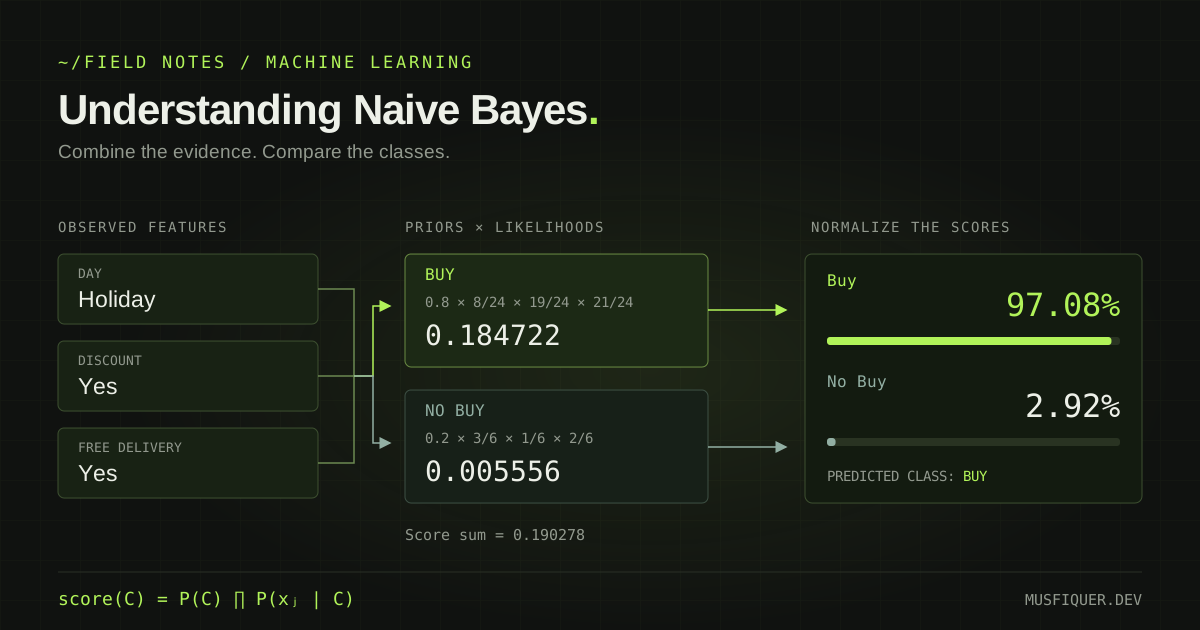
2. Calculate the Buy score
s(Buy) = P(Buy)
         × P(Holiday | Buy)
         × P(Discount = Yes | Buy)
         × P(Free delivery = Yes | Buy)

       = (24/30)(8/24)(19/24)(21/24)
       = 133 / 720
       ≈ 0.184722222
3. Calculate the No Buy score
s(No Buy) = (6/30)(3/6)(1/6)(2/6)
          = 1 / 180
          ≈ 0.005555556
The Buy score is larger. We could already select Buy, but these two scores are not the final class probabilities.
4. Normalize across the classes
Z = s(Buy) + s(No Buy)
  = 137 / 720
  ≈ 0.190277778

P_model(Buy | x) = (133/720) / (137/720)
                 = 133 / 137
                 ≈ 0.970802920

P_model(No Buy | x) = (1/180) / (137/720)
                    = 4 / 137
                    ≈ 0.029197080
The fitted model assigns 97.08% to Buy and 2.92% to No Buy for this input. These probabilities sum to one.
The normalization uses the sum of the class scores. Multiplying the overall marginal frequencies of Holiday, Discount, and Free delivery would introduce a separate assumption of independence across the full population. That assumption is not the same as independence conditional on Buy or No Buy.
The result is a model prediction, with uncertainty about whether its assumptions and learned frequencies describe future shopping behavior.
Explore the shopping classifier
Change the day and offer details to see the likelihood factors, class scores, and normalized results change. The two presets reproduce the holiday offer and a weekday with neither offer.
How do the features change the prediction?
INTERACTIVEChoose a shopping situation and inspect the factors behind each class score.
Predicted class: Buy
Normalize by the score sum: 0.190278
| Factor | Buy | No Buy |
|---|---|---|
| Prior | 24/30 | 6/30 |
| Day | 8/24 | 3/6 |
| Discount | 19/24 | 1/6 |
| Delivery | 21/24 | 2/6 |
For a weekday with no discount and no free delivery, the unsmoothed model assigns approximately 17.42% Buy and 82.58% No Buy. The prior still favors Buy, but the selected features provide enough evidence to reverse the decision.
The smoothing option keeps the class priors fixed and adds one to each feature-category count. Every category in this shopping table already has a positive count in both classes, so the toggle changes the estimates without repairing an existing zero.
Zero frequency and Laplace smoothing
In a categorical or token-count model, an estimated likelihood can be zero when a category or word never appears within a class. Multiplying by that zero removes the class from consideration, regardless of other evidence.
If all candidate scores become zero, normalization is undefined. If only one becomes zero, another class can still win, but the eliminated class may have been ruled out because of a small dataset rather than impossible evidence.
Additive smoothing adds a positive count α before calculating the distribution. For a categorical feature with K possible values and N_C training observations in class C:
P(xⱼ = v | C) = count(xⱼ = v, C) + α
                 ─────────────────────
                      N_C + αK
α = 1 is Laplace, or add-one, smoothing. The denominator includes one added count for every possible value. For Day, K = 3; for Discount and Free delivery, K = 2. 3
For example, the smoothed Holiday likelihood in No Buy becomes:
P(Holiday | No Buy, α = 1)
  = (3 + 1) / (6 + 3)
  = 4 / 9
Applying the same rule to every shopping feature yields approximately 95.42% Buy and 4.58% No Buy for the holiday offer. We have changed the estimated feature distributions, while preserving priors of 0.8 and 0.2.
The set of categories must be defined consistently. A completely new category may require an explicitly supported unknown category. Smoothing counts over known categories does not automatically expand an encoder's allowed values.
Worked example: classifying a short comment
For text, a common approach is Multinomial Naive Bayes. Each feature records how many times a vocabulary word occurs. Repeated occurrences contribute repeatedly to the score. 5
We will use five prepared training comments. Their token lists make the counting rule explicit:
| Row | Tokens after preprocessing | Class |
|---|---|---|
| A | check tube song channel | Spam |
| B | love song like channel | Spam |
| C | fan | Ham |
| D | song great love channel | Ham |
| E | love love love | Ham |
Assume a fixed vocabulary with eight words:
channel, check, fan, great, like, love, song, tube
The new comment is “I love song.” For this toy example, lowercase the text, remove punctuation and the common word I, and keep the resulting tokens love and song.
1. Estimate document priors
There are two Spam documents and three Ham documents:
P(Spam) = 2 / 5
P(Ham)  = 3 / 5
These are document counts. The word likelihoods below use token counts, which are a different denominator.
2. Count tokens within each class
| Word | Spam tokens | Ham tokens |
|---|---|---|
| channel | 2 | 1 |
| check | 1 | 0 |
| fan | 0 | 1 |
| great | 0 | 1 |
| like | 1 | 0 |
| love | 1 | 4 |
| song | 2 | 1 |
| tube | 1 | 0 |
| Total | 8 | 8 |
The three instances of love in row E contribute three counts. Treating that row as a single presence of the word would use a different representation.
3. Apply add-one smoothing
For a vocabulary V:
P(word | C) = token_count(word, C) + α
               ─────────────────────────
               total_tokens(C) + α|V|
With α = 1, both classes have denominator 8 + 8 = 16. The two likelihoods needed for the new comment are:
P(love | Spam) = (1 + 1) / (8 + 8) = 2/16
P(song | Spam) = (2 + 1) / (8 + 8) = 3/16

P(love | Ham)  = (4 + 1) / (8 + 8) = 5/16
P(song | Ham)  = (1 + 1) / (8 + 8) = 2/16
The vocabulary size is shared across classes. Each class's unsmoothed token total comes from its own documents. 4
The word fan shows why smoothing helps: its unsmoothed likelihood within Spam is 0/8, but add-one smoothing gives 1/16. This preserves a nonzero Spam score for a message containing that known vocabulary word. 8
4. Calculate and normalize the scores
The incoming comment contains love once and song once:
s(Spam) = (2/5)(2/16)(3/16)
        = 3 / 320
        = 0.009375000

s(Ham) = (3/5)(5/16)(2/16)
       = 3 / 128
       = 0.023437500

Z = 0.009375000 + 0.023437500
  = 0.032812500

P_model(Spam | comment) = 2 / 7 ≈ 0.285714286
P_model(Ham | comment)  = 5 / 7 ≈ 0.714285714
The model predicts Ham, assigning approximately 71.43% Ham and 28.57% Spam. That decision follows from the priors and token distributions in this particular corpus.
What happens when a word repeats?
If a test document contains a word t exactly n_t times, its likelihood contributes a power:
s(C) ∝ P(C) ∏ₜ P(t | C)ⁿᵗ
The model also loses word order under this representation. A different tokenizer, vocabulary, or treatment of negation can change the features and the result.
Computing safely with logarithms
A long document can require multiplying hundreds of small probabilities. Their product may become too small for floating-point arithmetic to represent accurately.
Compute a sum of log probabilities instead:
L(C) = log P(C) + Σₜ nₜ log P(t | C)
The logarithm is increasing, so the class with the highest log score also has the highest positive product score. For stable normalization:
m = max_C L(C)

P_model(C | x) = exp(L(C) − m)
                 ──────────────────
                 Σₖ exp(L(Cₖ) − m)
Subtracting the maximum keeps every exponential at most one while preserving the normalized result. Logarithms handle small products, while smoothing addresses zero likelihood estimates; they solve different numerical problems. 4
Types of Naive Bayes
Choose a variant whose feature distribution matches the representation:
| Variant | Feature representation | Example |
|---|---|---|
| Categorical | A finite set of categories per feature | Day type, discount, and delivery options |
| Multinomial | Nonnegative token or event counts | The comment example's word counts |
| Bernoulli | Binary presence or absence | Whether each vocabulary word appears |
| Gaussian | Continuous measurements, modeled with a normal distribution within each class | Numerical measurements for classification |
Categorical category indices identify labels rather than meaningful numeric distances. Word counts in Multinomial Naive Bayes record occurrences, while Bernoulli Naive Bayes explicitly includes absence as evidence. 3, 5, 6
Bernoulli: presence and absence
If xⱼ is 0 or 1 and qⱼ,C is the estimated probability of presence:
P(xⱼ | C) = qⱼ,C^(xⱼ) × (1 − qⱼ,C)^(1 − xⱼ)
When the feature is present, its factor is qⱼ,C. When it is absent, its factor is 1 − qⱼ,C. Repeating a word several times does not increase a binary presence feature. 6
Gaussian: continuous features
Gaussian Naive Bayes estimates a mean μⱼ,C and variance σ²ⱼ,C for each feature within each class. Its class-conditional likelihood uses the normal density:
f(xⱼ | C) = 1 / √(2πσ²ⱼ,C)
            × exp[−(xⱼ − μⱼ,C)² / (2σ²ⱼ,C)]
A density at a continuous value is not the probability of that exact value. Densities can exceed one; probabilities over intervals require integration. The relevant assumption concerns each feature within each class, rather than the overall pooled feature distribution. Variance smoothing helps avoid unstable calculations when an estimated variance is very small. 7
Other variants include Complement Naive Bayes, often considered for imbalanced text datasets. Selecting a name or distribution alone does not establish which model will perform best on a particular dataset. 2
Benefits, limitations, and evaluation
Why it can be a useful baseline
Naive Bayes estimates feature distributions separately within classes. That simplifies training and avoids estimating a large joint table of all feature combinations. For the shopping example, three day values and two binary features create 12 possible combinations, while the factorized model uses separate category counts.
Predictions combine a small set of learned quantities. The counts and likelihoods can be inspected directly, and the same approach naturally extends to more than two classes.
What needs checking
| Issue | Practical implication |
|---|---|
| Conditional dependence | Related features can provide overlapping evidence and distort class scores. |
| Sparse categories or words | Smoothing prevents observed zero counts from eliminating a class too readily. |
| Representation mismatch | A category label, word count, and continuous measurement need different likelihood models. |
| Class imbalance | Priors and error costs can affect useful decision rules. |
| Changing data | New vocabulary, customer behavior, or class frequencies can invalidate older estimates. |
| Probability calibration | A normalized output can be overconfident even when its predicted label is useful. |
A value such as 97.08% is a normalized probability under this fitted model. It is not evidence that 97.08% of future customers with these features will buy. Check calibration using independent predictions and outcomes when numerical probabilities matter. 9
Naive Bayes also has choices that can be tuned. These include additive smoothing strength, class priors, feature extraction, and Gaussian variance smoothing. The model's accuracy relative to logistic regression or an MLP depends on the dataset and evaluation; there is no universal ordering.
A practical evaluation sequence
- Separate training and evaluation data before learning counts, vocabulary, or preprocessing choices.
- Fit the feature representation and classifier using the training portion.
- Tune model choices using validation or cross-validation.
- Evaluate the final model on held-out examples, with attention to how future data will be collected. 11
For spam classification, inspect a confusion matrix and precision and recall. Accuracy alone can conceal poor behavior when one class dominates. If the numerical probabilities will guide decisions, also examine probability quality using calibration plots and an appropriate score such as log loss. 9, 10
Common uses include document-topic classification, spam filtering, and sentiment classification. A bag of words can miss order and negation, so preprocessing and feature choices remain part of the model.
Connecting this to the earlier models
The perceptron and MLP articles classify examples using weighted computations. Naive Bayes compares classes using priors and class-conditional feature models. Linear regression instead fits a numerical response.
For Naive Bayes, the central calculation is to estimate the prior and likelihood factors, combine them consistently, and normalize across classes when probabilities are needed. The independence assumption makes that calculation manageable; held-out evaluation tells us whether the resulting model is useful.
References
- M. Taboga, “Bayes' rule,” Lectures on probability theory and mathematical statistics, Kindle Direct Publishing, online appendix, 2021. Read the chapter.
- Scikit-learn developers, “Naive Bayes,” official documentation. Read the guide.
- Scikit-learn developers, “CategoricalNB,” official API documentation. Read the reference.
- C. D. Manning, P. Raghavan, and H. Schütze, Introduction to Information Retrieval, Cambridge University Press, 2008, section 13.2, “Naive Bayes text classification.” Read the chapter.
- Scikit-learn developers, “MultinomialNB,” official API documentation. Read the reference.
- Scikit-learn developers, “BernoulliNB,” official API documentation. Read the reference.
- Scikit-learn developers, “GaussianNB,” official API documentation. Read the reference.
- J. Starmer, “Naive Bayes, Clearly Explained!!!,” StatQuest, educational video. Watch the lesson.
- Scikit-learn developers, “Probability calibration,” official documentation. Read the guide.
- Scikit-learn developers, “Metrics and scoring: quantifying the quality of predictions,” classification metrics section, official documentation. Read the guide.
- Scikit-learn developers, “Cross-validation: evaluating estimator performance,” official documentation. Read the guide.