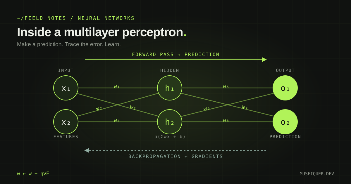
Understanding Multilayer Perceptrons: Forward Propagation and Backpropagation
Learn how an MLP predicts and learns, with a complete numerical example covering forward propagation, output and hidden-layer gradients, weight updates, and practical limitations.
A single perceptron makes a decision using a weighted sum and a threshold. A multilayer perceptron (MLP) connects several layers of artificial neurons, allowing it to learn relationships that a single linear decision boundary cannot capture.
The useful question is how those layers learn. We can answer it by following one small network through a prediction, calculating its error, and tracing that error backward through both the output layer and the hidden layer.
If inputs, weights, bias, and activation functions are new to you, start with the perceptron article.
In this article: Network structure · Activation and loss · Forward propagation · Output gradients · Hidden gradients · Weight updates · Benefits and limitations · References
What is a multilayer perceptron?
An MLP is a feedforward neural network with an input layer, one or more hidden layers, and an output layer. Its hidden neurons apply nonlinear activation functions to weighted sums of the values they receive. In supervised learning, labeled examples guide the adjustment of its weights and biases. 1, 11
Three ideas describe its structure:
- Input layer: receives features, such as pixel intensities or numerical measurements. These nodes provide values to the first hidden layer.
- Hidden layers: transform those values into intermediate representations. Each neuron calculates a weighted sum, adds a bias, and applies an activation function.
- Output layer: produces the values used for the task, such as class scores or a numerical prediction.
In a fully connected, or dense, layer, every neuron receives a connection from every neuron in the immediately preceding layer. An MLP does not require direct connections between every pair of layers. A dense transformation from n inputs to m neurons has n × m weights and, with one bias per destination neuron, m biases. 2, 4
Feedforward describes the prediction graph: information travels from inputs toward outputs without a recurrent cycle. Backpropagation calculates derivatives through that graph in reverse. It does not turn the prediction network into a recurrent network. 3
An MLP is the model architecture. Backpropagation is the method used to calculate gradients. Gradient descent is an optimization rule that uses those gradients to change parameters. These terms describe different parts of training.
Why hidden layers need nonlinearity
Stacking linear transformations alone produces another linear transformation. Nonlinear activations allow the network to combine features into relationships that cannot be represented by one linear map.
For a layer, the computation is:
zⱼ = Σᵢ wⱼᵢ aᵢ + bⱼ
aⱼ = f(zⱼ)

In matrix form:
z = W a + b
Here, aᵢ is an incoming value, wⱼᵢ is a connection weight, bⱼ is the destination neuron's bias, and f is its activation function.
An intuition: people recognizing a handwritten digit
Michael Stevens's The Stilwell Brain uses people acting as neurons to illustrate layered recognition. A handwritten digit is broken into small pieces. Early groups respond to simple visual features, later groups combine those features, and the final group identifies the digit. 5
The analogy helps explain how intermediate representations can build on one another. In a trained MLP, the representations are learned numerical transformations. We should not assume that each hidden neuron has an obvious label such as “vertical line” or “corner.”
Activation functions and loss functions
An activation function determines a neuron's output. A loss function measures how far the network's prediction is from the target. They have different jobs.
Choosing an activation
| Activation | Rule | Output range | Common role |
|---|---|---|---|
| Sigmoid | σ(z) = 1 / (1 + exp(−z)) | (0, 1) | Binary output, or an illustrative smooth neuron |
| Tanh | tanh(z) | (−1, 1) | A hidden activation with outputs centered around zero |
| ReLU | max(0, z) | [0, ∞) | Hidden layers |
| Softmax | pⱼ = exp(zⱼ) / Σₖ exp(zₖ) | Each value in (0, 1); the vector sums to 1 | Mutually exclusive multiclass outputs |
Sigmoid, tanh, and ReLU act on individual values. Softmax considers a vector of scores and normalizes it across classes. For a mutually exclusive classification task, the predicted class is commonly selected with argmax; every output value still exists before that decision. 6, 12
Choosing a loss
Let t represent a target and p a prediction. The following expressions describe one example; averaging across a dataset or batch adds an appropriate reduction.
| Loss | Expression | Common use |
|---|---|---|
| Mean squared error | (1 / m) Σⱼ (tⱼ − pⱼ)² | Regression |
| Binary cross-entropy | −[t ln(p) + (1 − t) ln(1 − p)] | Binary classification |
| Categorical cross-entropy | −Σⱼ tⱼ ln(pⱼ) | Mutually exclusive multiclass classification |
The negative sign in cross-entropy is necessary: a confident correct prediction should have a small loss. For one-hot targets, categorical cross-entropy reduces to the negative logarithm of the probability assigned to the correct class. 7, 8, 9
In implementations, check what a loss function expects. For example, PyTorch's CrossEntropyLoss takes unnormalized scores, or logits, and combines the required normalization with the loss calculation. Its BCEWithLogitsLoss similarly combines sigmoid and binary cross-entropy for numerical stability. 12
The numerical network we will train
We will use a small example adapted from Matt Mazur's backpropagation tutorial: two inputs, two hidden neurons, and two outputs. Every hidden and output neuron uses sigmoid. 10
Inputs:              x₁ = 0.05, x₂ = 0.10
Targets:             t₁ = 0.01, t₂ = 0.99
Hidden biases:       bₕ₁ = bₕ₂ = 0.35
Output biases:       bₒ₁ = bₒ₂ = 0.60
Learning rate:       η = 0.50
Activation:          σ(z) = 1 / (1 + exp(−z))
Keep the following connection map in mind throughout the calculation:
| Weight | Connection | Initial value |
|---|---|---|
w₁ | x₁ → h₁ | 0.15 |
w₂ | x₂ → h₁ | 0.20 |
w₃ | x₁ → h₂ | 0.25 |
w₄ | x₂ → h₂ | 0.30 |
w₅ | h₁ → o₁ | 0.40 |
w₆ | h₂ → o₁ | 0.45 |
w₇ | h₁ → o₂ | 0.50 |
w₈ | h₂ → o₂ | 0.55 |
Here, h₁ and h₂ will denote the hidden activations, and o₁ and o₂ the output activations. Their pre-activation values are written as zₕ₁, zₕ₂, zₒ₁, and zₒ₂.
The outputs in this example are independent sigmoid values. They are not a softmax probability distribution and do not need to sum to one. The purpose is to inspect a complete gradient calculation.
Displayed results are rounded to nine decimal places. Calculations use the unrounded values, so rounding an early activation and reusing it may produce a different final result.
Forward propagation step by step
1. Calculate the hidden activations
For the first hidden neuron:
zₕ₁ = w₁x₁ + w₂x₂ + bₕ₁
    = (0.15 × 0.05) + (0.20 × 0.10) + 0.35
    = 0.3775

h₁ = σ(0.3775)
   ≈ 0.593269992
For the second hidden neuron:
zₕ₂ = w₃x₁ + w₄x₂ + bₕ₂
    = (0.25 × 0.05) + (0.30 × 0.10) + 0.35
    = 0.3925

h₂ = σ(0.3925)
   ≈ 0.596884378
2. Calculate the output activations
The hidden activations become the inputs to the output layer:
zₒ₁ = w₅h₁ + w₆h₂ + bₒ₁
    ≈ 1.105905967
o₁  = σ(zₒ₁) ≈ 0.751365070

zₒ₂ = w₇h₁ + w₈h₂ + bₒ₂
    ≈ 1.224921404
o₂  = σ(zₒ₂) ≈ 0.772928465
The network currently predicts approximately [0.751365070, 0.772928465]. We want [0.01, 0.99], so the first output should decrease and the second should increase.
3. Calculate the total error
For this example, use half the sum of squared output errors:
E = ½(t₁ − o₁)² + ½(t₂ − o₂)²

E₁ ≈ 0.274811083
E₂ ≈ 0.023560026
E  ≈ 0.298371109
With exactly two outputs, this expression equals their mean squared error. The distinction matters when the number of outputs changes: half the sum and the mean use different scaling factors. Our derivative below follows the expression written here.
Backpropagation through the output layer
We need to know how a weight affects E. For w₅, the chain of dependencies is:
w₅ → zₒ₁ → o₁ → E
The chain rule multiplies the derivatives along that path:
∂E/∂w₅ = (∂E/∂o₁)(∂o₁/∂zₒ₁)(∂zₒ₁/∂w₅)
Each term has a straightforward meaning.
How the error changes with the output: differentiating the squared error gives o₁ − t₁.
∂E/∂o₁ = o₁ − t₁
        ≈ 0.741365070
How sigmoid changes with its input: its derivative is the activation multiplied by one minus that activation.
∂o₁/∂zₒ₁ = o₁(1 − o₁)
          ≈ 0.186815602
How the weighted sum changes with the weight: since zₒ₁ = w₅h₁ + w₆h₂ + bₒ₁, the derivative with respect to w₅ is h₁.
Putting those terms together:
∂E/∂w₅ = (o₁ − t₁)o₁(1 − o₁)h₁
        ≈ 0.082167041
This is the local slope of the loss with respect to w₅ at the current parameters. For a sufficiently small change, ΔE ≈ 0.082167041 × Δw₅. It describes sensitivity near the current point.
Reusing the output deltas
Write δₒⱼ = ∂E/∂zₒⱼ. The delta collects the error derivative and activation derivative at an output neuron:
δₒ₁ = (o₁ − t₁)o₁(1 − o₁) ≈  0.138498562
δₒ₂ = (o₂ − t₂)o₂(1 − o₂) ≈ −0.038098237
Each incoming weight gradient is the destination neuron's delta multiplied by the incoming activation:
| Weight | Gradient | Value |
|---|---|---|
w₅ | δₒ₁h₁ | 0.082167041 |
w₆ | δₒ₁h₂ | 0.082667628 |
w₇ | δₒ₂h₁ | −0.022602540 |
w₈ | δₒ₂h₂ | −0.022740242 |
The signs fit the desired direction: subtracting the positive gradients decreases w₅ and w₆, while subtracting the negative gradients increases w₇ and w₈.
Backpropagation through the hidden layer
The hidden neurons have no target values of their own. Their gradients come from the effect they have on later neurons.
Crucially, h₁ influences both o₁ and o₂. Its error derivative must include both paths. The same is true for h₂. 10
1. Collect both error paths for h₁
The first output contributes δₒ₁w₅, and the second contributes δₒ₂w₇:
∂E/∂h₁ = δₒ₁w₅ + δₒ₂w₇
        ≈ (0.138498562 × 0.40)
          + (−0.038098237 × 0.50)
        ≈ 0.055399425 − 0.019049118
        ≈ 0.036350306
The two paths pull in opposite directions. We add their contributions before continuing through h₁'s activation.
2. Apply the hidden activation derivative
∂h₁/∂zₕ₁ = h₁(1 − h₁)
          ≈ 0.241300709

δₕ₁ = (δₒ₁w₅ + δₒ₂w₇)h₁(1 − h₁)
     ≈ 0.008771355
This delta measures how the total loss changes with the first hidden neuron's pre-activation value.
3. Calculate w₁ and w₂ gradients
zₕ₁ = w₁x₁ + w₂x₂ + bₕ₁, so its derivatives with respect to w₁ and w₂ are x₁ and x₂:
∂E/∂w₁ = δₕ₁x₁
        ≈ 0.008771355 × 0.05
        ≈ 0.000438568

∂E/∂w₂ = δₕ₁x₂
        ≈ 0.008771355 × 0.10
        ≈ 0.000877135
The full chain rule for w₁ is therefore:
∂E/∂w₁ = [δₒ₁w₅ + δₒ₂w₇] × h₁(1 − h₁) × x₁
4. Repeat the calculation for h₂
The connections from h₂ to the outputs are w₆ and w₈:
∂E/∂h₂ = δₒ₁w₆ + δₒ₂w₈
        ≈ (0.138498562 × 0.45)
          + (−0.038098237 × 0.55)
        ≈ 0.041370323

δₕ₂ = (δₒ₁w₆ + δₒ₂w₈)h₂(1 − h₂)
     ≈ 0.009954255

∂E/∂w₃ = δₕ₂x₁ ≈ 0.000497713
∂E/∂w₄ = δₕ₂x₂ ≈ 0.000995425
The general hidden-layer rule
For hidden neuron j, sum over every neuron k receiving its output:
δⱼ = f′(zⱼ) Σₖ wₖⱼδₖ

Gradient of an incoming weight:
∂E/∂wⱼᵢ = δⱼaᵢ
The first expression collects downstream effects. The second attributes that delta to an individual incoming connection. Repeating these calculations layer by layer extends backpropagation to networks with multiple hidden layers.
Use the original weights from this forward pass when calculating every gradient. Replacing w₅ or w₇ with an updated value while computing the hidden gradients would mix two different parameter states.
Updating all eight weights
Gradient descent changes a weight using:
w_new = w_old − η × ∂E/∂w
With η = 0.5, the complete update is:
| Weight | Old value | Gradient | New value |
|---|---|---|---|
w₁ | 0.150000000 | 0.000438568 | 0.149780716 |
w₂ | 0.200000000 | 0.000877135 | 0.199561432 |
w₃ | 0.250000000 | 0.000497713 | 0.249751144 |
w₄ | 0.300000000 | 0.000995425 | 0.299502287 |
w₅ | 0.400000000 | 0.082167041 | 0.358916480 |
w₆ | 0.450000000 | 0.082667628 | 0.408666186 |
w₇ | 0.500000000 | −0.022602540 | 0.511301270 |
w₈ | 0.550000000 | −0.022740242 | 0.561370121 |
For example, w₁_new = 0.15 − 0.5 × 0.000438567734… ≈ 0.149780716.
All eight gradients were calculated before any weight was changed. For this particular update, we hold the hidden biases at 0.35 and the output biases at 0.60 so the effect of changing the weights is easy to inspect.
Bias gradients
A trainable bias participates in the same computation as a weight on a constant input of 1. Consequently:
∂E/∂bⱼ = δⱼ
bⱼ_new = bⱼ_old − ηδⱼ
For example, updating independent biases from the same original forward pass would give bₕ₁_new ≈ 0.345614323 and bₒ₁_new ≈ 0.530750719. Each hidden and output neuron normally has its own bias; equal initial values do not require those parameters to remain tied together. If a model deliberately shares one bias across several neurons, the shared parameter's gradient is the sum of their deltas.
The check below uses the weight-only update in the table, with biases unchanged.
Run a fresh forward pass
Recalculate both hidden activations and both output activations using the new weights:
Before the update:
o₁ ≈ 0.751365070
o₂ ≈ 0.772928465
E  ≈ 0.298371109

After the update, biases fixed:
o₁ ≈ 0.742088111
o₂ ≈ 0.775284968
E  ≈ 0.291027774
The first prediction has moved downward and the second upward. The loss has decreased. This is one training step on one example; it does not establish performance on unseen data.
Learning rate and the training loop
The learning rate scales the parameter change. A large value can overshoot a useful region or make training unstable. A very small value can make progress slow. Gradient descent uses the learning rate; selecting it is a separate tuning decision. Schedules and adaptive optimizers can vary effective step sizes during training.
A typical iteration follows this sequence:
- Run a forward pass on an example or batch.
- Calculate a scalar loss using the targets.
- Backpropagate to calculate gradients at the current parameters.
- Let an optimizer update the weights and trainable biases.
- Repeat, monitoring validation performance as well as training loss.
One epoch is a pass through the training dataset. With batches, an epoch contains multiple parameter updates. Training should be assessed with held-out data; repeatedly fitting the same example cannot show that a model generalizes.
Benefits, limitations, and applications
What an MLP can do well
Nonlinear hidden layers can model interactions between features and support both classification and regression. Increasing width or depth changes the model's capacity. Dense computations can also be expressed as matrix operations, making them suitable for parallel execution.
The universal approximation result explains part of this flexibility: under suitable activation and capacity assumptions, a feedforward network can approximate continuous functions on a compact input domain to arbitrary accuracy. It is an expressive-capacity result, with no guarantee that a particular training run will find the necessary parameters or generalize well. 13
Problems to watch for
| Problem | Why it matters |
|---|---|
| Overfitting | A large network can fit noise or memorize training examples. Regularization and validation help assess generalization. |
| Parameter and memory cost | Dense layers create many weights as input dimensions and layer widths grow. |
| Hyperparameter sensitivity | Depth, width, learning rate, initialization, and training duration affect results. |
| Non-convex optimization | Training can encounter different local minima, saddle points, or flat regions. |
| Weak or unstable gradients | Saturating activations and long chains of derivatives can make learning difficult. |
| Feature scaling | Large differences in feature magnitudes can make optimization harder. |
| Interpretability | Hidden representations may be difficult to explain in terms of familiar input features. |
| Data quality | Incorrect labels, leakage, or an unrepresentative dataset can undermine evaluation. |
These are reasons to evaluate an MLP carefully against simpler baselines. They do not disappear just because more layers are added. 1, 11
Where the model can be useful
The same architecture can be adapted to different tasks by choosing suitable input features, output representations, and losses:
| Task | Example input | Possible output |
|---|---|---|
| Classification | Customer or transaction features | A class score or probability |
| Regression | Numerical measurements | A continuous prediction |
| Pattern recognition | Pixels or extracted visual features | A class prediction |
| Speech or language classification | Audio features or text representations | A category or score |
| Forecasting | Measurements from a fixed window of past observations | A future value |
| Recommendation or anomaly scoring | Features describing a user, item, or event | A relevance or anomaly score |
MLPs have a long history in atmospheric modeling, and dense neural models are also useful in systems working with language and audio features. The choice of architecture still depends on the task. A plain MLP does not automatically encode spatial structure or sequence order; those must be represented in its features or handled by other parts of the system. 1, 14, 15
The main idea to keep
Forward propagation transforms inputs into a prediction. Backpropagation traces how the loss depends on each parameter. A hidden neuron learns through the sum of the effects it has on downstream neurons, and an optimizer uses those gradients to update the model.
Once that hidden-layer calculation is clear, the larger network is a repetition of the same weighted sums, activation derivatives, and chain-rule steps.
References
- M. W. Gardner and S. R. Dorling, “Artificial neural networks (the multilayer perceptron)—a review of applications in the atmospheric sciences,” Atmospheric Environment, vol. 32, nos. 14–15, pp. 2627–2636, 1998. DOI: 10.1016/S1352-2310(97)00447-0.
- Saturn Cloud, “What is a feedforward fully connected neural network and how to implement it in Matlab,” online article, n.d. Read the article.
- Brilliant, “Feedforward Neural Networks,” online learning resource, n.d. Read the resource.
- P. Mahajan, “Fully Connected vs Convolutional Neural Networks,” The Startup, Medium, October 23, 2020. Read the article.
- Vsauce, “The Stilwell Brain,” Mind Field, season 3, episode 3, video featuring Michael Stevens. Watch the episode.
- GeeksforGeeks, “Activation functions in neural networks,” online article, n.d. Read the article.
- Wikipedia contributors, “Mean squared error,” online encyclopedia entry. Read the entry.
- D. Shah, “Understanding Binary Cross-Entropy and Log Loss for Effective Model Monitoring,” Aporia, August 17, 2023; currently hosted by Coralogix. Read the article.
- Neural Threads, “Categorical cross-entropy loss—the most important loss function,” Medium, n.d. Read the article.
- M. Mazur, “A Step by Step Backpropagation Example,” March 17, 2015. Source of the numerical network and the output- and hidden-layer gradient walkthrough. Read the tutorial.
- Scikit-learn developers, “Neural network models (supervised),” official documentation. Read the guide.
- PyTorch contributors, official activation and loss documentation: Softmax, MSELoss, BCEWithLogitsLoss, and CrossEntropyLoss.
- K. Hornik, M. Stinchcombe, and H. White, “Multilayer feedforward networks are universal approximators,” Neural Networks, vol. 2, no. 5, pp. 359–366, 1989. DOI: 10.1016/0893-6080(89)90020-8.
- M. D. Mohanty and M. N. Mohanty, “Verbal sentiment analysis and detection using recurrent neural network,” in Advanced Data Mining Tools and Methods for Social Computing, Academic Press, pp. 85–106, 2022. DOI: 10.1016/B978-0-32-385708-6.00012-6.
- A. Singhal and D. K. Sharma, “Voice signal-based disease diagnosis using IoT and learning algorithms for healthcare,” in Implementation of Smart Healthcare Systems using AI, IoT, and Blockchain, Academic Press, pp. 59–81, 2023. DOI: 10.1016/B978-0-323-91916-6.00005-9.