Understanding Linear Regression: Fitting a Line, Measuring Error, and Making Predictions
Learn how linear regression fits data, with worked pizza-price and multiple-regression examples, an interactive fitting graph, error metrics, and a gradient descent calculation.
How much should a pizza cost if we know its diameter? A linear regression model answers this kind of question by learning a relationship between input features and a numerical output.
The calculation starts with a familiar expression: a weighted input plus an intercept. We will fit a line to three pizza prices, extend the method to two predictors, and calculate how prediction errors guide learning.
The examples are small enough to work through by hand. They illustrate the method rather than establish a pricing rule or the performance of a real business model.
In this article: The model · Pizza-price example · Interactive fit · Error metrics · Gradient descent · Multiple regression · Model checks · References
What is linear regression?
Regression models predict numerical responses from input features. For example, a response might be a price, a measurement, or a future demand value. The features are the information available when making that prediction.
Linear regression models the response as a linear combination of features. In ordinary least squares, fitting means selecting coefficients that minimize the sum of squared differences between observed and predicted values. 1
Simple linear regression
With one predictor, the fitted model is a straight line:
ŷ = wx + b
| Symbol | Meaning | In the pizza example |
|---|---|---|
x | Input feature or predictor | Diameter in inches |
y | Observed response or target | Actual price in dollars |
ŷ | Predicted response | Estimated price in dollars |
w | Slope or fitted coefficient | Dollars per additional inch |
b | Intercept | The line's prediction when diameter is zero |
The hat in ŷ distinguishes the prediction from the observed value y. Different texts use m, β₁, or a₁ for the slope. We will use w here, keeping the notation close to weights in neural networks.
For a statistical description, we can write y = β₀ + β₁x + ε, where ε represents variation the model does not explain. The fitted line estimates the response's conditional mean under the model. Individual observations can fall above or below it. 2
Multiple linear regression
With several predictors, the expression becomes:
ŷ = β₀ + β₁x₁ + β₂x₂ + … + βₚxₚ
Each coefficient describes the fitted change associated with one predictor while the others remain fixed. A two-predictor model describes a plane in three-dimensional input-response space. More predictors extend the same calculation to higher dimensions.
“Linear” refers to the coefficients. A model such as ŷ = β₀ + β₁x + β₂x² can trace a curve in x while remaining linear in its fitted parameters. Choosing transformed features changes the relationships the model can represent. 3
Worked example: predicting pizza prices
Suppose we have these three illustrative observations:
Diameter x (inches) | Price y (dollars) |
|---|---|
| 8 | 10 |
| 10 | 13 |
| 12 | 16 |
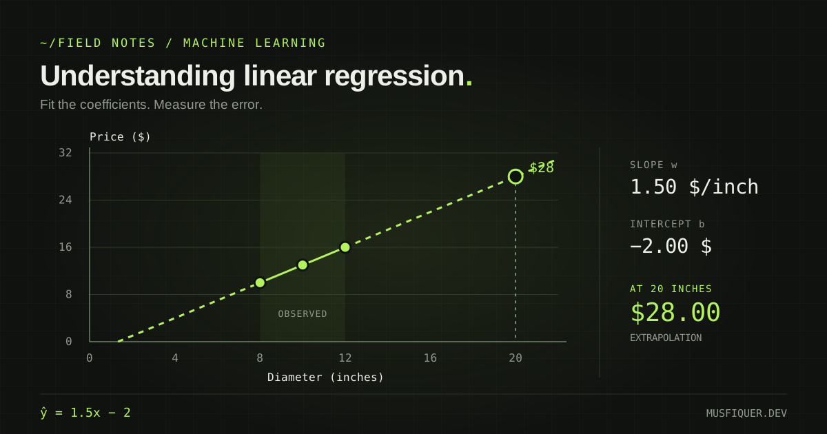
We want to fit ŷ = wx + b, then estimate the price of a 20-inch pizza.
1. Calculate the means
x̄ = (8 + 10 + 12) / 3 = 10
ȳ = (10 + 13 + 16) / 3 = 13
The least-squares line with an intercept passes through (x̄, ȳ). To find its slope, compare how each input and target deviates from its mean. 2
2. Calculate the slope
For inputs that are not all identical:
w = Σᵢ (xᵢ − x̄)(yᵢ − ȳ)
    ───────────────────────
         Σᵢ (xᵢ − x̄)²
Build the terms explicitly:
xᵢ | yᵢ | xᵢ − x̄ | yᵢ − ȳ | Product of deviations | Squared input deviation |
|---|---|---|---|---|---|
| 8 | 10 | −2 | −3 | 6 | 4 |
| 10 | 13 | 0 | 0 | 0 | 0 |
| 12 | 16 | 2 | 3 | 6 | 4 |
| Sum | 12 | 8 |
Therefore:
w = 12 / 8 = 1.5
The fitted price increases by $1.50 for each additional inch of diameter within this model.
3. Calculate the intercept
b = ȳ − wx̄
  = 13 − (1.5 × 10)
  = −2

Fitted model:
ŷ = 1.5x − 2
An intercept of −2 is part of the fitted line. It does not imply that a shop sells a zero-inch pizza for negative money. Zero is outside the observed diameter range, so that interpretation has no useful support here.
4. Make a prediction
For a 20-inch pizza:
ŷ = (1.5 × 20) − 2
  = 28 dollars
The model's prediction is $28. Its training predictions are $10, $13, and $16, exactly matching the three observations.
This dataset lies perfectly on a line. Real observations usually contain noise, and the least-squares line generally leaves nonzero residuals.
Interpolation and extrapolation
A prediction at x = 11 stays within the observed range of 8–12 inches. It is an interpolation, giving ŷ = $14.50.
The prediction at x = 20 is an extrapolation. It extends the learned relationship beyond the observed range. The arithmetic is valid, but the relationship might change for larger pizzas. Ingredients, area, and a shop's pricing policy could matter. A perfect training fit does not establish that this extrapolated price will be accurate. 3
Explore the fitted line
Move the slope and intercept to see the line change. The vertical residual segments show the gap between each observed price and the current prediction. Select Fit the data to restore the least-squares solution.
What makes a line fit?
INTERACTIVEAdjust the coefficients and compare the predictions with the observed prices.
The highlighted band marks the observed diameter range. The dashed extension and hollow marker identify the extrapolated prediction. Training MSE uses only the three observed pizzas, so changing the prediction at 20 inches does not directly add a fourth training error.
Residuals and error metrics
A residual is an observed value minus its fitted prediction:
eᵢ = yᵢ − ŷᵢ
A positive residual means the model predicted too low. A negative residual means it predicted too high.
For N observations, several quantities summarize those differences:
| Quantity | Expression | Interpretation |
|---|---|---|
| Mean residual | (1 / N) Σᵢ eᵢ | Average signed difference; positive and negative errors can cancel |
| MAE | (1 / N) Σᵢ abs(eᵢ) | Mean absolute error, in the target's units |
| MSE | (1 / N) Σᵢ eᵢ² | Mean squared error, in squared target units |
| RMSE | √[(1 / N) Σᵢ eᵢ²] | Root mean squared error, in the target's units |
Squaring makes large residuals count more heavily. Absolute values also prevent cancellation, with a different penalty shape. RMSE takes the square root of MSE, which restores the original measurement units. 4
For a quick example, suppose two residuals are +2 and −2 dollars:
Mean residual = (2 − 2) / 2 = 0 dollars
MAE           = (2 + 2) / 2 = 2 dollars
MSE           = (4 + 4) / 2 = 4 dollars²
RMSE          = √4         = 2 dollars
The zero mean residual does not indicate perfect predictions. Both predictions missed their targets.
The training cost and the factor of one-half
An ordinary least-squares model minimizes squared error. A convenient training objective is:
J(w, b) = (1 / 2N) Σᵢ (wxᵢ + b − yᵢ)²
This objective is half the prediction MSE. The factor of one-half simplifies its derivatives. Multiplying the same squared-error objective by a positive constant does not change the minimizing coefficients, although it changes gradient magnitudes and the learning-rate scale.
We will keep MSE = SSE / N and J = MSE / 2 distinct. Here, SSE is the sum of squared residuals. Statistics texts also use “mean square error” for an error-variance estimate that divides SSE by residual degrees of freedom. Check the denominator before comparing those quantities. 2
What does R² measure?
For nonconstant targets, the coefficient of determination compares the model with predicting the evaluation set's target mean:
R² = 1 − SSE / SST
SST = Σᵢ (yᵢ − ȳ)²
For the pizza data, SSE = 0 and SST = 18, so training R² = 1. On new data, R² can be negative when predictions are worse than the mean baseline on that evaluation set. Neither a high R² nor a small training MSE establishes causation or generalization. 4
Learning with gradient descent
The pizza slope formula gives a direct solution. We can also learn coefficients iteratively by calculating derivatives and following the negative gradient. This is the same optimization idea used in the MLP article. 5
For the half-MSE objective above:
∂J/∂w = (1 / N) Σᵢ (wxᵢ + b − yᵢ)xᵢ
∂J/∂b = (1 / N) Σᵢ (wxᵢ + b − yᵢ)

w_new = w_old − η × ∂J/∂w
b_new = b_old − η × ∂J/∂b
The expressions use prediction − target. That is the negative of our residual convention, target − prediction, and follows from differentiating the squared loss.
One complete update
Use a smaller dataset to inspect the cost:
Observations:  (1, 1), (2, 2), (3, 3)
Model:         ŷ = wx
Initial slope: w = 0.5
Learning rate: η = 0.1
For this example, fix the intercept at zero. We are updating only w.
xᵢ | yᵢ | Prediction 0.5xᵢ | Prediction minus target | Squared error |
|---|---|---|---|---|
| 1 | 1 | 0.5 | −0.5 | 0.25 |
| 2 | 2 | 1.0 | −1.0 | 1.00 |
| 3 | 3 | 1.5 | −1.5 | 2.25 |
The starting cost is:
J(0.5) = (0.25 + 1.00 + 2.25) / 6
       = 7 / 12
       ≈ 0.583333333
Now calculate the gradient:
∂J/∂w = [(−0.5 × 1) + (−1.0 × 2) + (−1.5 × 3)] / 3
       = −7 / 3
       ≈ −2.333333333

w_new = 0.5 − 0.1 × (−7 / 3)
      = 11 / 15
      ≈ 0.733333333
Use that updated slope in a fresh prediction and loss calculation:
New predictions ≈ [0.733333333, 1.466666667, 2.200000000]

J(w_new) = 112 / 675
         ≈ 0.165925926
The cost decreased. For this particular dataset, yᵢ = xᵢ, so we can express the entire cost curve as:
J(w) = (7 / 3)(w − 1)²
Its minimum is at w = 1, where every training prediction is correct and J = 0.
Squared-error linear regression has a convex objective in its coefficients. A suitable learning rate lets gradient descent approach a minimum. Large steps can overshoot, and feature scaling affects the size of the gradients. If predictors are linearly dependent, minimizing coefficients may be nonunique. 5, 6
Worked example: multiple linear regression
Consider four illustrative observations with two predictors. These small numbers let us follow the matrix calculation without assigning them a business interpretation:
| Row | x₁ | x₂ | Target y |
|---|---|---|---|
| A | 1 | 4 | 1 |
| B | 2 | 5 | 6 |
| C | 3 | 8 | 8 |
| D | 4 | 2 | 12 |
The model is ŷ = β₀ + β₁x₁ + β₂x₂. Every observation contributes an equation, and the fit finds coefficients that minimize their total squared residual.
1. Construct the design matrix
Include a column of ones for the intercept:
    ┌ 1  1  4 ┐       ┌  1 ┐       ┌ β₀ ┐
X = │ 1  2  5 │   y = │  6 │   β = │ β₁ │
    │ 1  3  8 │       │  8 │       └ β₂ ┘
    └ 1  4  2 ┘       └ 12 ┘

Predictions: ŷ = Xβ
Rows are observations. Columns are the intercept feature and the two predictors. We seek the coefficient vector β minimizing ‖Xβ − y‖².
2. Form the normal equations
Setting the squared-error gradient to zero gives:
XᵀXβ = Xᵀy
For these observations:
       ┌  4  10   19 ┐         ┌  27 ┐
XᵀX = │ 10  30   46 │   Xᵀy = │  85 │
       └ 19  46  109 ┘         └ 122 ┘
For example, the last component of Xᵀy is (4 × 1) + (5 × 6) + (8 × 8) + (2 × 12) = 122.
The normal equations are therefore:
 4β₀ + 10β₁ +  19β₂ =  27
10β₀ + 30β₁ +  46β₂ =  85
19β₀ + 46β₁ + 109β₂ = 122
3. Solve for the coefficients
Eliminate β₀ from the second and third equations. After scaling, the remaining pair is:
10β₁ −  3β₂ =  35
−6β₁ + 75β₂ = −25
From the first equation, β₁ = 3.5 + 0.3β₂. Substitute that into the second:
−6(3.5 + 0.3β₂) + 75β₂ = −25
                 73.2β₂ = −4

β₂ = −10 / 183  ≈ −0.054644809
β₁ = 425 / 122  ≈  3.483606557
β₀ = −311 / 183 ≈ −1.699453552
The fitted model is:
ŷ ≈ −1.699453552 + 3.483606557x₁ − 0.054644809x₂
Displayed coefficients are rounded. The predictions below use the unrounded solution.
4. Check the predictions and residuals
| Row | Actual y | Predicted ŷ | Residual y − ŷ |
|---|---|---|---|
| A | 1 | 1.565574 | −0.565574 |
| B | 6 | 4.994536 | 1.005464 |
| C | 8 | 8.314208 | −0.314208 |
| D | 12 | 12.125683 | −0.125683 |
SSE ≈ 1.445355191
MSE = SSE / 4 ≈ 0.361338798
The fit leaves residuals because the four observations do not lie exactly on this fitted plane. The coefficients describe associations within this toy dataset, with each predictor considered while the other is held fixed.
There are four observations and three fitted parameters. This is enough to illustrate the algebra, with only one residual degree of freedom. It gives little evidence about performance on future observations.
The matrix formula and numerical practice
When X has full column rank, the solution can be written:
β̂ = (XᵀX)⁻¹Xᵀy
The inverse requires that rank condition. Duplicate or exactly dependent feature columns make it unavailable. Even near dependence can make coefficients sensitive to small data changes.
The formula explains the solution, but explicitly forming and inverting XᵀX can worsen numerical conditioning. In code, use a least-squares solver based on QR or singular value decomposition rather than implementing a matrix inverse by hand. Libraries also provide solutions when the coefficients are not uniquely identified. 6, 7
Assumptions and model checks
Calculating a line is only part of the work. We also need to decide whether its structure and predictions suit the data.
| Check | What to look for |
|---|---|
| Mean relationship | Curvature in a residual plot can indicate missing transformations or interactions. |
| Dependence between observations | Time patterns or clustering can undermine usual independence assumptions. |
| Error variance | A widening residual spread can indicate nonconstant variance. |
| Unusual observations | Outliers and high-leverage points can strongly affect a squared-error fit. |
| Feature dependence | Strongly related predictors can make individual coefficients unstable. |
| Evaluation data | Use observations that were not used to fit or select the model. |
Residual plots help check whether unexplained structure remains. Classical standard errors and inference rely on additional assumptions about errors. Normal-error assumptions support familiar exact small-sample tests and intervals, but normality is not required simply to calculate the least-squares fit. 8
Keep two distinctions in mind:
- Association and causation: a fitted coefficient describes a conditional association. Causal interpretation requires a defensible study design and assumptions about confounding.
- Training fit and prediction quality: a low training error does not tell us the error on new examples. Fit preprocessing on training data, then assess the model on held-out data. For time-dependent prediction, preserve the relevant time ordering. 9
Benefits, limitations, and applications
Linear regression gives an interpretable baseline for numerical prediction. Coefficients have a direct meaning within the chosen feature representation, and fitting is well supported by statistical and numerical tools.
Its limitations follow from those choices. A simple line can miss curved relationships. Squared loss is sensitive to unusual observations. Adding many predictors relative to the available data can overfit, and correlated predictors can make coefficients unstable.
Ridge regression adds an L2 coefficient penalty. Lasso adds an L1 penalty and can set some coefficients to zero. These methods change the fitting objective. Their strength should be selected using validation, rather than assumed to improve every dataset. 6
Examples of tasks that can be framed as numerical prediction include:
| Task | Possible predictors | Numerical response |
|---|---|---|
| Demand estimation | Price, promotions, seasonal features | Units sold |
| Property modeling | Size, location features, building age | Sale price |
| Environmental modeling | Weather and measured conditions | A continuous environmental measurement |
| Sports analysis | Training and past performance features | A performance measurement |
| Health research | Relevant measured covariates | A continuous outcome |
These are possible modeling setups, not evidence that a linear model is best for each task. Feature choices, study design, data quality, and evaluation determine whether the model is useful.
Connecting the model to neural networks
Linear regression uses the same weighted-sum structure introduced in the perceptron article. Its output is a numerical prediction. The binary perceptron applies a threshold to produce a class decision.
An MLP combines weighted sums with nonlinear hidden activations to represent more complex relationships. Across these models, the useful questions remain concrete: what is predicted, how is error measured, how are parameters fitted, and how well does the result work on new data?
References
- Scikit-learn developers, “LinearRegression,” official API documentation. Read the reference.
- Pennsylvania State University, “Simple Linear Regression,” STAT 501: Regression Methods, online course notes. Read the lesson.
- NIST/SEMATECH, “Linear Least Squares Regression,” e-Handbook of Statistical Methods, section 4.1.4.1. Read the chapter.
- Scikit-learn developers, “Metrics and scoring: quantifying the quality of predictions,” regression metrics section, official documentation. Read the guide.
- Google, “Linear regression: Gradient descent,” Machine Learning Crash Course. Read the lesson.
- Scikit-learn developers, “Linear Models,” ordinary least squares, Ridge, and Lasso sections, official documentation. Read the guide.
- SciPy contributors, “scipy.linalg.lstsq,” official API documentation. Read the reference.
- NIST/SEMATECH, “Check of assumptions,” e-Handbook of Statistical Methods, section 5.2.4.5. Read the chapter.
- Scikit-learn developers, “Cross-validation: evaluating estimator performance,” official documentation. Read the guide.